• Running pyCapsid remotely on Google Colab
  • Colab quick-start guide
  • Video Tutorials
    • Running the pyCapsid Colab Notebook
    • Visualizing the results in ChimeraX
  • Colab output example
• Locally via Jupyter Notebook
  • Fetch and load PDB
  • Build ENM Hessian
  • Perform NMA
  • Predict, fit, and compare b-factors
  • Perform quasi-rigid cluster identification (QRC)
  • Visualize in ChimeraX
  • Visualize in Jupyter Notebook with nglview
• Running pyCapsid using a simple config.toml file
  • A simple config.toml example
  • pyCapsid config.toml parameters
• Visualizing saved results
• ProDy Integration

Running pyCapsid remotely on Google Colab

The simplest way to use pyCapsid is using this colab notebook which runs pyCapsid on a free Google cloud-based platform in a Jupyter environment. The Colab notebook is self documenting and is designed to be simple to use. The Colab notebook has built in methods for visualizing the results for small structures using NGLView, but we recommend installing molecular visualization software UCSF ChimeraX locally for high-quality visualizations of larger structures. The following quick-start guide is also included in the notebook.

Colab quick-start guide

Follow the steps described below to obtain the dominant dynamics and quasi-rigid units of a protein complex. To help navigate the guide, we recommend displaying the Colab notebook’s Table of contents (open the View menu on the top bar and choose Table of contents):

1. Specify the structure to be analyzed in the Input structure section. Run the code block to set the parameters and, if not fetching a remote structure, upload the structure file.
2. Modify the default pyCapsid parameters if necessary in the pyCapsid parameters section. Run the code block to set the parameters.
3. Execute the rest of the notebook by navigating the Colab menu Runtime and choosing the option Run all or Run after in the cell after the pyCapsid parameters. This will install pyCapsid, run the pipeline, and generate and store the results.
   • The pipeline will automatically compress and download the outputs in two zip files. Your browser might prompt a request to allow the downloading process. pyCapsid_report.zip contains key results, a report summarizing them, and instructions for visualizing the results in ChimeraX. pyCapsid_results.zip contains all of the relevant data files created by pyCapsid and a readme describing their contents.
   • If you encounter any issues in the downloading process, check the section Problems downloading results?
   • The execution time and maximum size of the protein complex depend on the computing power and memory of the Colab cloud service used, which depends on the user’s Colab plan. The section Estimate time and memory gives an estimate of the time and memory requirements based on the number of residues in the structure.
4. Extract and read the downloaded report (pyCapsid_report.*) for a summary and interpretation of the main results. The report is available in three formats: Markdown, *.md, Microsoft Word (*.docx), and Web page’s HyperText Markup Language (*.html). The multi-formatted report aims to facilitate users adapting pyCapsid’s results to their publication needs. Check the section pyCapsid report for further details.
   • Additional results are displayed throughout the different subsections in the Run the pyCapsid pipeline’s section.
5. The 3D images of the protein complex will be missing in pyCapsid_report.*. You will need to generate them using ChimeraX. We recommend downloading and installing ChimeraX from here. To visualize the quasi-rigid domains obtained, open a new session in ChimeraX and run the following instruction in the command line to open a file browser in ChimeraX:

   runscript browse
   

   Then, inside the browser, navigate in the pyCapsid_report/ChimeraX/ folder and open the script chimerax_script_colab.py. This will generate a 3D model of the protein complex coloring the quasi-rigid domains in ChimeraX and store snapshots in the folder pyCapsid_report/figures/structures/ that will be visible in the .html and .md reports. To generate an animation of the dynamics of the lowest-frequency non-degenerate mode, start a new ChimeraX session and follow the same steps above, but opening instead the script chimerax_script_animate_mode.py.

6. Optionally, read the section Generate advanced analysis to learn how to obtain advanced analyses using results stored during the execution of the pyCapsid pipeline.

Video Tutorials

Running the pyCapsid Colab Notebook

Visualizing the results in ChimeraX

Colab output example

An example of what the completed pyCapsid_report.md downloaded by the notebook will look like is shown here.

Locally via Jupyter Notebook

This tutorial covers the step by step use pyCapsid to identify the quasi-rigid subunits of an example capsid. This tutorial also comes in the form of a Jupyter notebook for those who wish to run it locally. The example notebook is also provided for local use in the notebooks folder.

Once the package and other dependencies are installed, download the notebook and run the following command in its directory to launch Jupyter Notebook.

jupyter notebook

Fetch and load PDB

This code acquires the pdb file from the RCSB databank, loads the necessary information, and saves copies for possible use in visualization in other software.

from pyCapsid.PDB import getCapsid
pdb = '4oq8'
capsid, calphas, asymmetric_unit, coords, bfactors, chain_starts, title = getCapsid(pdb)

Build ENM Hessian

This code builds a hessian matrix using an elastic network model defined by the given parameters. The types of model and the meaning of the parameters are provided in the documentation.

from pyCapsid.CG import buildENMPreset
kirch, hessian = buildENMPreset(coords, preset='U-ENM')

Perform NMA

This code calculates the n lowest frequency modes of the system by calculating the eigenvalues and eigenvectors of the hessian matrix.

from pyCapsid.NMA import modeCalc
evals, evecs = modeCalc(hessian)

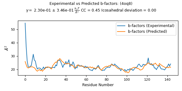
Predict, fit, and compare b-factors

This code uses the resulting normal modes and frequencies to predict the b-factors of each alpha carbon, fits these results to experimental values from the pdb entry, and plots the results for comparison.

from pyCapsid.NMA import fitCompareBfactors
evals_scaled, evecs_scaled, cc, gamma, n_modes = fitCompareBfactors(evals, evecs, bfactors, pdb)

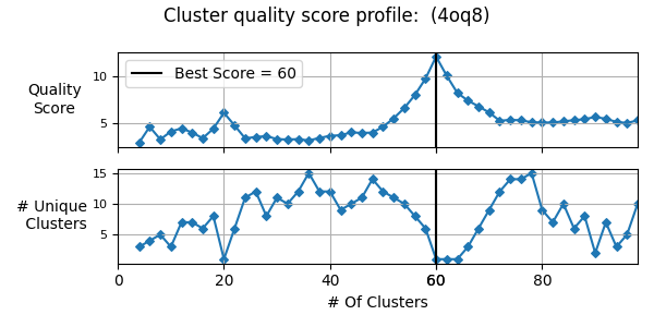
Perform quasi-rigid cluster identification (QRC)

from pyCapsid.NMA import calcDistFlucts
from pyCapsid.QRC import findQuasiRigidClusters

dist_flucts = calcDistFlucts(evals_scaled, evecs_scaled, coords)

cluster_start = 4
cluster_stop = 100
cluster_step = 2
labels, score, residue_scores  = findQuasiRigidClusters(pdb, dist_flucts, cluster_start=cluster_start, cluster_stop=cluster_stop, cluster_step=cluster_step)

Visualize in ChimeraX

If ChimeraX (https://www.cgl.ucsf.edu/chimerax/download.html) is installed you may provide a path to the chimerax executable file to automatically visualize the results in chimerax. This is done using the runscript command in chimerax and this python script: (https://github.com/luquelab/pyCapsid/blob/main/src/pyCapsid/scripts/chimerax_script.py).

from pyCapsid.VIS import chimeraxViz
chimeraxViz(labels, pdb, chimerax_path='C:\\Program Files\\ChimeraX\\bin')

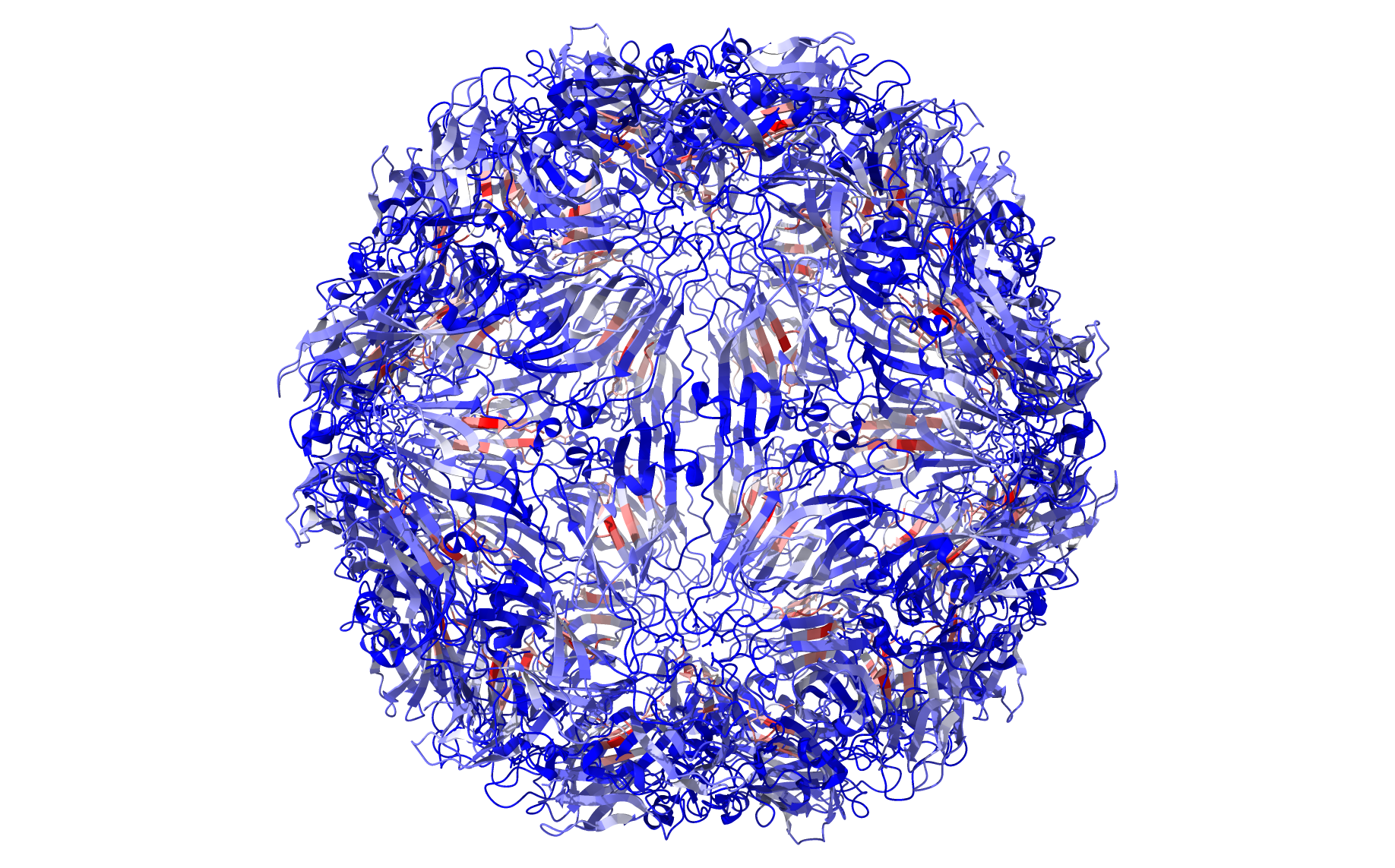
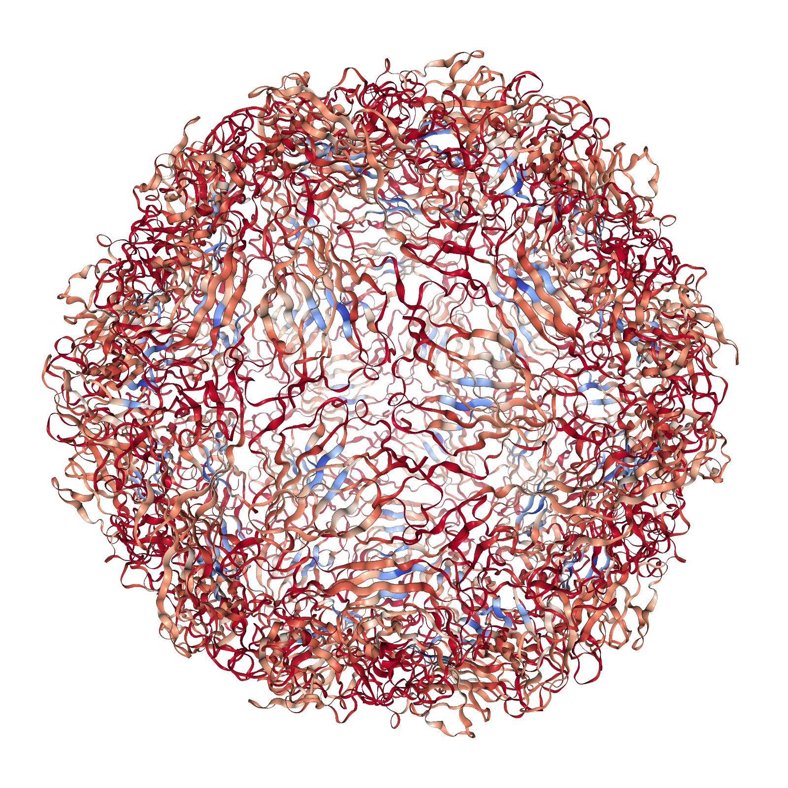
Running the same code but replacing labels with residue_scores and adding rwb_scale=True visualizes the quality score of each residue. This is a measure of how rigid each residue is with respect to its cluster. Blue residues make up the cores of rigid clusters, and red residues represent borders between clusters.

from pyCapsid.VIS import chimeraxViz
chimeraxViz(residue_scores, pdb, chimerax_path='C:\\Program Files\\ChimeraX\\bin', rwb_scale=True)

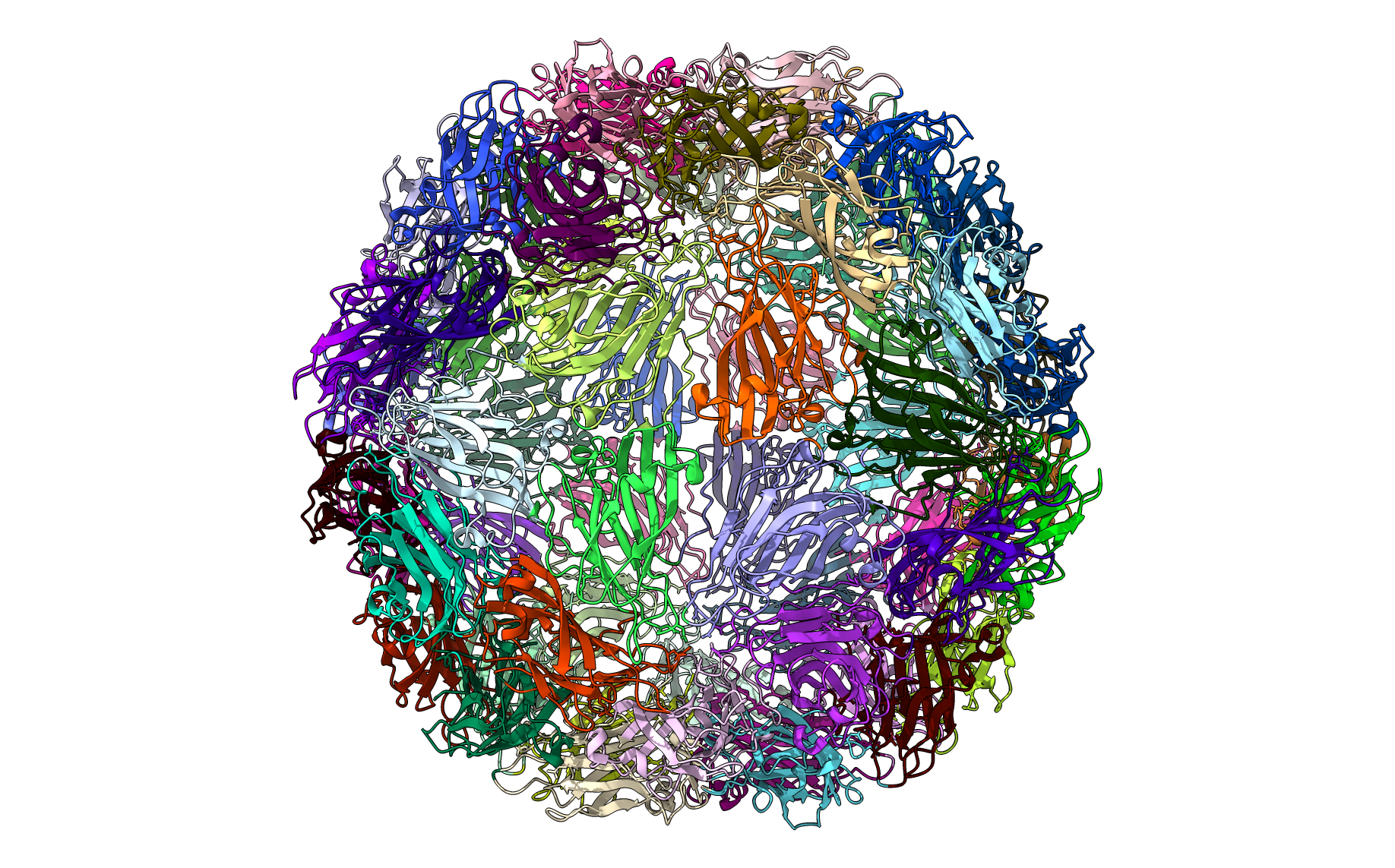
Visualize in Jupyter Notebook with nglview

You can visualize the results in a Jupyter notebook with nglview. The following function returns an NGLView view with the results colored based on cluster. See the nglview documentation for further info on how to create high quality images. (http://nglviewer.org/nglview/release/v2.7.7/index.html)

This cell will create a standard view of the capsid, which the next cell will modify to create the final result.

from pyCapsid.VIS import createCapsidView
view_clusters = createCapsidView(pdb, capsid)
view_clusters

Do not run this cell until the above cell has finished rendering. If the above view doesn’t change coloration, run this cell again.

from pyCapsid.VIS import createClusterRepresentation
createClusterRepresentation(pdb, labels, view_clusters)
# Add rep_type='spacefill' to represent the atoms of the capsid as spheres. This provides less information regarding the proteins but makes it easier to identify the geometry of the clusters
#createClusterRepresentation(pdb, labels, view_clusters, rep_type='spacefill')

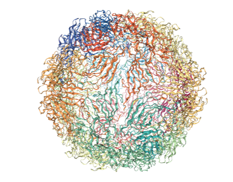
This should result in the following image: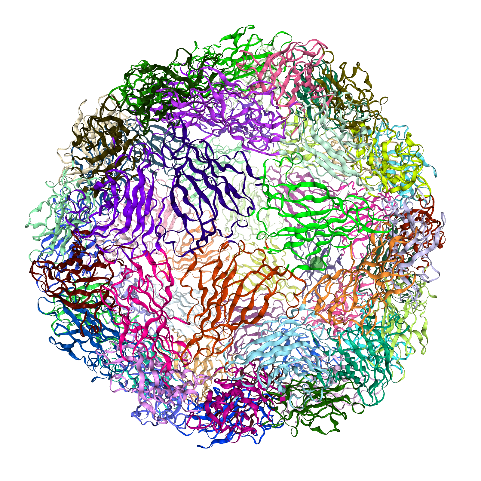

If the above view doesn’t change coloration, run the cell again. In general do not run the cell until the first cell has finished rendering.

Once you’ve done this use this code to download the results

view_clusters.center()
view_clusters.download_image(factor=2)

Running the same code but replacing labels with residue_scores and adding rwb_scale=True visualizes the quality score of each residue. This is a measure of how rigid each residue is with respect to its cluster. Blue residues make up the cores of rigid clusters, and red residues represent borders between clusters.

# This code adds a colorbar based on the residue scores
print('Each atom in this structure is colored according to the clustering quality score of its residue.')
import matplotlib.colorbar as colorbar
import matplotlib.pyplot as plt
from pyCapsid.VIS import clusters_colormap_hexcolor
import numpy as np
hexcolor, cmap = clusters_colormap_hexcolor(residue_scores, rwb_scale=True)
fig, ax = plt.subplots(figsize=(10, 0.5))
cb = colorbar.ColorbarBase(ax, orientation='horizontal',
                            cmap=cmap, norm=plt.Normalize(np.min(residue_scores), np.max(residue_scores)))
plt.show()

# This cell will create an empty view, which the next cell will 
# modify to create the final result.
from pyCapsid.VIS import createCapsidView
view_scores = createCapsidView(pdb, capsid)
view_scores

from pyCapsid.VIS import createClusterRepresentation
createClusterRepresentation(pdb, residue_scores, view_scores, rwb_scale=True)

view_scores.center()
view_scores.download_image(factor=2)

Running pyCapsid using a simple config.toml file

This tutorial also has a corresponding example notebook. This is a simpler and faster way to run the entire pyCapsid pipeline as outlined in the colab notebook and save the results by setting the parameters ahead of time in a text file. To do this download this example from our GitHub or copy and paste the following into a text editor and save the output as ‘config.toml’

A simple config.toml example

[PDB]
pdb = '4oq8' # PDB ID of structure
save_all_path = './4oq8' # where to save the results

[CG]
preset = 'U-ENM' # Model Preset To Use
save_hessian = true # Whether to save the hessian matrix

[NMA]
n_modes = 200 # Number of low frequency modes to calculate
eigen_method = 'eigsh' # eigen method to use

[b_factors]
fit_modes = true # Whether to select the number of modes used to maximize correlation

[QRC]

[VIS]
method = 'chimerax'
chimerax_path = 'C:\Program Files\ChimeraX\bin\ChimeraX.exe'

[plotting]

Once you’ve created the ‘config.toml’ file, the following python code will run the entire pyCapsid pipeline using the specified settings. Make sure to either run python in the same directory as the config file or properly include the path to the file in the python code.

from pyCapsid import run_capsid_report
run_capsid_report('config.toml')

pyCapsid config.toml parameters

• PDB
  • pdb (string) - PDB id of entry to download. If local is True, then the filename of a local file.
  • pdbx (true/false) - Whether the target structure should be acquired in pdbx/mmcif format.
  • local (true/false) - Whether to instead use a local file
  • assembly_id (integer) - specifies the biological assembly. If not set it defaults to 1. If no assembly info is provided in the structures set this value to None.
• CG
  • preset specifies the elastic network model used to coarse-grained the protein complex. There are four different models that can be specified. Each model sets certain parameters. Additional parameters can be provided to modify the models. Read the API documentation for buildENM to see the parameters.
    • ANM: Anisotropic network model with a default cutoff of 15Å and no distance weighting.
    • GNM: Gaussian network model (no three-dimensional directionality) with a default cutoff of 7.5Å and no distance weighting.
    • U-ENM: Unified elastic network Model with a default cutoff of 7.5Å and a default anisotropy parameter (f_anm) of 0.1. It is the default and recommended option.
    • bbENM: Backbone-enhanced Elastic network model with a default cutoff of 7.5Å and no distance weighting.
    • none: Use specific parameters set in the config file. Read the API documentation for buildENM to see the parameters.
  • save_hessian (true/false) - Whether to save the resulting hessian matrix.
• NMA
  • n_modes (integer) - specifies the number of modes to be used to calculate the dynamics. Must be an integer. The default value is 200. However, while using 200 modes can yield good results, we recommend using more modes for larger structures. Increasing the number of modes often improves the accuracy but results in longer computational times. The fit_modes option described below can assist in selecting the optimal value for this parameter.
  • eigen_method What method to use to calculate the lowest-frequency modes. Three available methods.
    • eigsh: scipy.sparse.linalg.eigsh with shift_invert. Default CPU method. Set the parameter shift_invert = false when using this for reduced performance and better memory usage.
    • lobpcg: scipy.sparse.linalg.lobpcg. Less memory intensive than eigsh, but can be slower and has less precise results for symmetric structures.
    • lobcuda: cupyx.scipy.sparse.linalg.lobpcg. CUDA accelerated lobpcg, requires CUDA and cupy package.
• b_factors
  • fit_modes (true/false) - If true pyCapsid will select the number of low-frequency modes used in further calculations by finding the number of modes (less than n_modes) that results in the best correlation with experimental B-factors. If true pyCapsid will also provide a plot showing how correlation with B-factors changes with the number of modes used. If false, all modes calculated will be used.
  • force_ico (true/false) - If true use a number of modes that result in icosahedrally symmetric squared fluctuations.
  • ico_tol (float) - Acceptable deviation in icosahedral symmetry if force_ico is true.
• QRC
  • cluster_start (integer) - specifies the minimum number of clusters used in the clustering analysis to identify the optimal quasi-rigid mechanical units. The minimum value is 3.
  • cluster_stop (integer) - specifies the maximum number of clusters used in the clustering analysis to identify the optimal quasi-rigid mechanical units. The number of residues in the structure represents an upper value. The default value is 100. The recommended value should be at least the number of proteins in the structure. Ideally, the value should be the number of proteins times the number of expected protein domains defining the protein fold.
  • cluster_step (integer) - specifies the steps taken when exploring the range of clusters to determine the optimal quasi-rigid mechanical units. The default value is 2. It is recommended to refine the search in a sub-region once a potential optimal result has been identified.
  • fluct_cutoff (float) - When calculating distance fluctuations, only calculate them for residues within a cutoff distance in angstroms. Larger values will bias the results towards larger clusters. Default is 7.5.
  • cluster_method What method to use to cluster the embedded points.
    • discretize: Adapted from scikit-learn function based on a clustering method specifically for spectral clustering described in Multiclass Spectral Clustering
    • kmeans: sklearn.cluster.k_means. A more general clustering method.
  • score_method How to determine the quality score of each cluster.
    • median: Use the median quality score of each residue in the cluster.
    • mean: Use the mean quality score of each residue in the cluster.
• VIS
  • method How to visualize the results for the full capsid:
    • chimerax: Using ChimeraX. If chimerax_path is set correctly this will automatically open ChimeraX and visualize the results.
    • nglview: Only works in a jupyter notebook environment. Uses NGLView to create an interactive widget in the notebook.
  • chimerax_path: Complete path to the chimerax executable if using method = 'chimerax'.
  • offscreen (true/false) - If true use the offscreen rendering option of ChimeraX. This allows for the visualization of results on a system without a built-in display. Only works on Linux.
• plotting
  • suppress_plots (true/false) - Suppress interactive plots while running pyCapsid.

[PDB]
pdb = '4oq8'
pdbx = false
local = false
assembly_id = 1
save_all_path = './4oq8'

[CG]
preset = 'U-ENM'
save_hessian = true

[NMA]
n_modes = 200
eigen_method = 'eigsh'
shift_invert = true

[b_factors]
fit_modes = true
force_ico = false
ico_tol = 0.002

[QRC]
cluster_start = 10
cluster_stop = 100
cluster_step = 2
fluct_cutoff = 7.5
cluster_method = 'discretize'
score_method = 'median'

[VIS]
method = 'chimerax'
chimerax_path = 'C:\Program Files\ChimeraX\bin\ChimeraX.exe'
offscreen = false

[plotting]
suppress_plots = true

Visualizing saved results

The numerical results are saved as compressed .npz files by default and can be opened and used to visualize the results afterwards. This includes the ability to visualize clusters that weren’t the highest scoring cluster. In this example we visualize the results of clustering the capsid into 20 clusters.

from pyCapsid.VIS import visualizeSavedResults
results_file = f'4oq8_final_results_full.npz' # Path of the saved results
labels_20, view_clusters_20 = visualizeSavedResults('4oq8', results_file, n_cluster=20, method='nglview')
view_clusters_20

from pyCapsid.VIS import createClusterRepresentation
createClusterRepresentation('4oq8', labels_20, view_clusters_20)

ProDy Integration

ProDy is a free and open-source Python package for protein structural dynamics analysis. Our ENM and NMA modules make performance improvements compared to ProDy, but it still has a large number of useful applications of ENM/NMA results. Luckily one can make use of pyCapsids faster ENM and NMA module while still being able to use ProDy’s other features by performing the calculations using pyCapsid and passing the results to ProDy.

from prody import ANM, parsePDB
capsid = parsePDB('7kq5', biomol=True)
calphas = capsid.select('protein and name CA')
anm = ANM('T. maritima ANM analysis')

from pyCapsid.CG import buildENM
coords = calphas.getCoords()
kirch, hessian = buildENM(coords, cutoff=10)

from pyCapsid.NMA import modeCalc
evals, evecs = modeCalc(hessian)

anm._hessian = hessian
anm._array = evecs
anm._eigvals = evals